 |
49 (12) (1997), pp. 14-19. JOM is a publication of The Minerals, Metals & Materials Society |
|---|
|
49 (12) (1997), pp. 14-19. JOM is a publication of The Minerals, Metals & Materials Society |
|---|
| CONTENTS |
|---|
|
|
Enormous progress has been made in the calculation of phase diagrams during the past 30 years. This progress will continue as model descriptions are improved and computational technology advances. Improvement has been made in the model descriptions in the CALPHAD method, the coupling of phase diagrams with kinetic process modeling, computer programs for easy access to phase diagram information, and the construction of databases used for calculating the phase diagrams of complex commercial alloys.
Phase diagrams are visual representations of the state of a material as a function of temperature, pressure, and concentrations of the constituent components and are, therefore, frequently hailed as basic blueprints or roadmaps for alloy design, development, processing, and understanding. The importance of phase diagrams is also reflected by the publication of such handbooks as Binary Alloy Phase Diagrams,1 Phase Equilibria, Crystallographic and Thermodynamic Data of Binary Alloys,2 Phase Equilibrium Diagrams,3 which continues in Phase Diagrams for Ceramists,4 Handbook of Ternary Alloy Phase Diagrams,5 and Ternary Alloys.6
The state of a two-component material at constant pressure can be presented in the well-known graphical form of binary phase diagrams. For three-component materials, an additional dimension is necessary for a complete representation. Therefore, ternary systems are usually presented by a series of sections or projections. Due to their multidimensionality, the interpretation of the diagrams of more complex systems can be quite cumbersome for an occasional user of these diagrams. For systems with more than three components, the graphical representation of the phase diagram in a useful form becomes not only a challenging task, but is also hindered by the lack of sufficient experimental information. However, the difficulty of graphically representing systems with many components is irrelevant for the calculation of phase diagrams; such calculations can be customized for the materials problem of interest.
While it is only modern developments in modeling and computational technology that have made computer calculations of multicomponent phase equilibria a realistic possibility, the correlation between thermodynamics and phase equilibria was established more than a century ago by J.W.Gibbs, whose groundbreaking work has been summarized by Hertz.7 Although the mathematical foundation was laid, more than 30 years passed before J.J. van Laar8 published his mathematical synthesis of hypothetical binary systems. To describe the solution phases, van Laar used concentration dependent terms that Hildebrand9 called regular solutions. More than 40 years had passed when J.L.Meijering published his calculations of miscibility gaps in ternary10 and quaternary solutions.11 Shortly afterward, Meijering applied this method to the thermodynamic analysis of the Cr-Cu-Ni system.12 Simultaneously, Kaufman and Cohen13 applied thermodynamic calculations in the analysis of the martensitic transformation in the Fe-Ni system; Kaufman continued his work on the calculation of phase diagrams, including pressure dependence. In 1970, Kaufman and Bernstein14 summarized the general features of the calculation of phase diagrams and also gave listings of computer programs for the calculation of binary and ternary phase diagrams, thus laying the foundation for the CALPHAD method (CALculation of PHAse Diagrams). In 1973, Kaufman organized the first project meeting of the international CALPHAD group. Since then, the CALPHAD group has grown consistently larger.
Another important paper on the calculation of phase equilibria was published in the 1950s. In his paper, Kikuchi15 described a method to treat order/disorder phenomena. This method later became known as the cluster variation method (CVM) and is extensively used in conjunction with first-principles calculations. Although these calculations are computationally very intensive, enormous progress in algorithms and computer speed has been made in recent years. The predicted phase diagrams are generally topologically correct, but they currently lack sufficient accuracy for practical applications. De Fontaine16 gives an extensive review of these calculations.
| FIGURES |
|---|
|
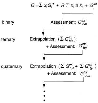
Figure 1: CALPHAD methodology. The assessed excess Gibbs energies of the constituent subsystems are for extrapolation to a higher component system.
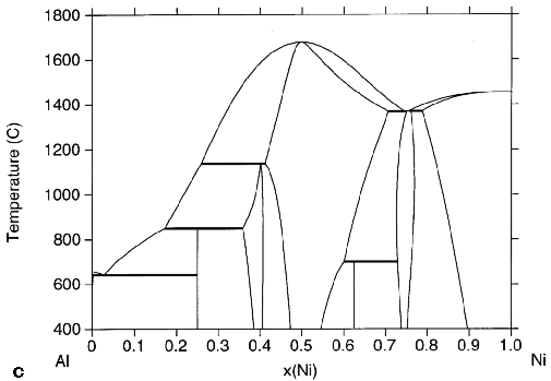
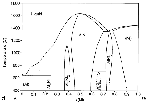
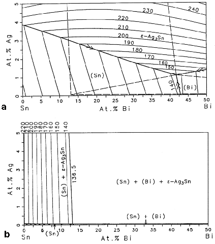
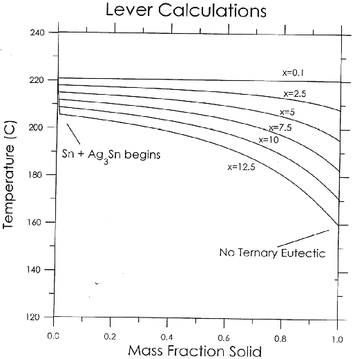
Figure 2: Different assessments of the Al-Ni system showing the progress made with the CALPHAD method: (Figure 2a) a 1978 assessment by Kaufman and Nesor,47 (Figure 2b) a 1988 assessment by Ansara et al.,38 (Figure 2c) a 1997 assessment by Ansara et al.,39 and (Figure 2d) the evaluated experimental diagram.48 Figure 3: BA tin-rich corner of the Sn-Bi-Ag system with isotherms showing (a) the liquidus surface (dashed lines are the boundaries of the three-phase equilibria at the eutectic temperature) and (b) the solidus surface. Figure 4: Temperature vs. calculated fraction solid curves for six Sn-3.5Ag-xBi (in weight percent) alloys using (Figure 4a) Lever rule calculations and (Figure 4b) Scheil calculations. Figure 5: Phase fraction vs. temperature curves for solidification of alloy Al-4.44Cu-1.56Mg-0.55Mn-0.23Fe-0.21Si-0.05Zn (in weight percent) using (Figure 5a) Lever rule calculation and (Figure 5b) Scheil calculation. Figure 6: Fraction solid vs. local temperature curves for the two nodes from the casting simulation compared to the curves obtained from Scheil and Lever rule solidification calculations. |
The experimental determination of phase diagrams is a time-consuming and costly task. This becomes even more pronounced as the number of components increases. The calculation of phase diagrams reduces the effort required to determine equilibrium conditions in a multicomponent system. A preliminary phase diagram can be obtained from extrapolation of the thermodynamic functions of constituent subsystems. This preliminary diagram can be used to identify composition and temperature regimes where maximum information can be obtained with minimum experimental effort. This information can then be used to refine the original thermodynamic functions.
Numerical phase diagram information is also frequently needed in other modeling efforts. Even though phase diagrams represent thermodynamic equilibrium, it is well established that the phase equilibria can be applied locally (local equilibrium) to describe the interfaces between phases. In such cases, only the concentrations at this interface are assumed to obey the requirements of thermodynamic equilibrium. Thermodynamic modeling of phase diagrams and kinetic modeling have been successfully coupled for a variety of processes, such as carburizing/nitriding,19,20 diffusion couples,21-23 dissolution of precipitates,24,25 and solidification.26,27 Phase-equilibrium calculations can not only give the phases present and their compositions, but can also provide numerical values of enthalpy contents, temperature, and concentration dependence of phase boundaries for coupling of microscopic and macroscopic modeling. Banerjee et al.28 give an example of such a coupling of phase-equilibria calculations and solidification micromodels in a macroscopic heat and fluid-flow analysis of a casting.
In recent years, the expression "computational thermodynamics" is frequently used in place of "calculation of phase diagrams." This reflects the fact that the phase diagram is only a portion of the information that can be obtained from these calculations.
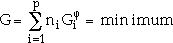 |
(1) |
where ni is the number of moles, and  is the Gibbs energy of phase i.
A thermodynamic description of a system requires the assignment of thermodynamic functions for each phase. The CALPHAD method employs a variety of models to describe the temperature, pressure, and concentration dependencies of the free-energy functions of the various phases. The contributions to the Gibbs energy of a phase j can be written as
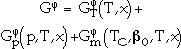 |
(2) |
where  is the contribution to the Gibbs energy by the temperature (T) and the composition (x),
  is the contribution of the pressure (p), and
 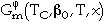 is the magnetic contribution of the Curie or Néel temperature (TC) and the average magnetic moment per atom (
 0).
0).
The temperature dependence of the concentration term of  is usually expressed as a power series of T.
 |
(3) |
where a, b, c, and dn are coefficients, and n are integers. To represent the pure elements, the n are typically 2, 3, -1, and 7 or -9.29 This function is valid for temperatures above the Debye temperature; in each of the equations in the following models describing the concentration dependence, the G coefficients on the right-hand side can have such a temperature dependence. Frequently, only the first two terms are used for the representation of the excess Gibbs energy. Dinsdale29 also gives expressions for the effects of pressure and magnetism on the Gibbs energy; however, pressure dependence for condensed systems at normal pressures is usually ignored.
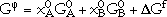
For multicomponent systems, it has proven useful to distinguish three contributions from the concentration dependence to the Gibbs energy of a phase,  .
.
 |
(4) |
The first term, G0, corresponds to the Gibbs energy of a mechanical mixture of the constituents of the phase; the second term, Gideal, corresponds to the entropy of mixing for an ideal solution, and the third term, Gxs, is the so-called excess term. Since Hildebrand9 introduced the term "regular solution" to describe interactions of different elements in a random solution, a series of models have been proposed for phases that deviate from this regularity (i.e., show a strong compositional variation in their thermodynamic properties) to describe the excess Gibbs energy. For example, an ionic liquid model30 or associate model,31 among others, have been proposed for liquid phases. For ordered solid phases, Wagner and Schottky32 introduced the concept of defects on the crystal lattice in order to describe deviations from stoichiometry.
A description of order/disorder transformations was proposed by Bragg and Williams.33 Since then, many other models have been proposed. Today, the most commonly used models (listed in order of increasing complexity) are those for stoichiometric phases, regular solution-type models for disordered phases, and sublattice models for ordered phases having a range of solubility or exhibiting an order/disorder transformation. The following examples give descriptions of models for binary phases and can easily be expanded for ternary and higher order phases.
The Gibbs energy of a binary stoichiometric phase is given by
 |
(5) |
where  and
and  are mole fractions of elements A and B and are given by the stoichiometry of the compound,
  and
and  are the respective reference states of elements A and B, and
  Gf is the Gibbs energy of formation. The first two terms correspond to G0, and the third term corresponds to Gxs in Equation 4. Gideal of Equation 4 is zero for a stoichiometric phase, since there is no random mixing.
Binary solution phases, such as liquid and disordered solid solutions, are described as random mixtures of the elements by a regular-solution type model
 |
(6) |
where xA and xB are the mole fractions, and and are the reference states of elements A and B, respectively. The first two terms correspond to G0 and the third term, from random mixing, to Gideal in Equation 4. The Gi of the fourth term are coefficients of the excess Gibbs energy term, Gxs, in Equation 4. The sum of the terms (xA - xB)i is the so-called Redlich-Kister polynomial,34 which is the most commonly used polynomial in regular-solution type descriptions. Although other polynomials have been used in the past, in most cases they can be converted to Redlich-Kister polynomials.35
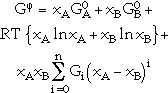
The most complex and general model is the sublattice model frequently used to describe ordered binary solution phases. The basic premise for this model is that a sublattice is assigned for each distinct site in the crystal structure. For example, the CsCl (B2) structure consists of two sublattices, one of which is occupied predominantly by Cs atoms and the other by Cl atoms. An ordered binary solution phase with two sublattices that exhibits substitutional deviation from stoichiometry can be described by the expression
 |
(7) |
where  , and
, and  are the species concentrations of element A and B on sublattices 1 and 2 with
  ,
,  and
and  . a1 and a2 are the site fractions of the sublattices 1 and 2 and are given by the number of sites in the unit cell. The first two terms correspond to G0, and the third term corresponds to Gideal in Equation 4. The remaining terms are the excess Gibbs energy term, Gxs, in Equation 4. The coefficients
  , and
, and  can be visualized as the Gibbs energies of the end-member phases. The end-member phases are formed when each sublattice is occupied only by one kind of species and can be either real (
 : A atoms on sublattice 1 and B atoms on sublattice 2) or hypothetical (
 , and
, and  ). The remaining terms of Gxs describe interactions between the atoms on one sublattice similar to regular-solution type models for disordered solution phases. This model description was first introduced by Sundman and Ågren36 and later refined by Andersson et al.37
For the treatment of order/disorder transformations with this model, the coefficients in Gxs are not independent of each other. For example, Ansara et al.38 derived dependencies for the order/disorder transformation of fcc/L12. This model was later modified by Ansara et al.39 to allow independent evaluation of the thermodynamic properties of the disordered phase. Chen et al.40 have proposed another model for the treatment of ordered phases.
It should be noted that Equations 5 and 6 are, in fact, special cases of Equation 7. Equation 7 reduces to Equation 6 if only one sublattice is considered or to Equation 5 if only one species is considered on each of the two sublattices. The generality of the sublattice description allows the formulation of a general description for multicomponent phases that can easily be computerized. Lukas et.al.35 give an example of a description.
From the condition that the Gibbs energy at thermodynamic equilibrium reveals a minimum for given temperature, pressure, and composition, J.W. Gibbs derived the well-known equilibrium conditions that the chemical potential,  , of each component, n, is the same in all phases,
 |
(8) |
The chemical potentials are related to the Gibbs energy by the well known equation
 |
(9) |
Equation 8 results in n nonlinear equations that can be used in numerical calculations. All of the CALPHAD-type software tools use methods like the two-step method of Hillert41 or the one-step method of Lukas et al.35 to minimize the Gibbs energy. The equations obtained from these methods are usually nonlinear and are solved numerically using a Newton-Raphson technique.
 |
(10) |
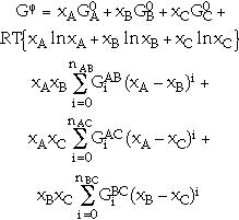
where the parameters  have the same values as in Equation 6 for each of the binary systems. If necessary, a ternary term xA xB xC GABC(T,x) can be added in order to describe the contribution of three element interactions to the Gibbs energy.
The usual strategy for assessment of a multicomponent system is shown in Figure 1. First, the thermodynamic descriptions of the constituent binary systems are derived. Thermodynamic extrapolation methods are then used to extend the thermodynamic functions of the binaries into ternary and higher order systems. The results of such extrapolations can then be used to design critical experiments. The results of the experiments are compared to the extrapolation, and if necessary, interaction functions are added to the thermodynamic description of the higher order system. As mentioned previously, the coefficients of the interaction functions are optimized on the basis of these data. In principle, this strategy is followed until all 2, 3,... n constituent systems of an n-component system have been assessed. However, experience has shown that, in most cases, no corrections or very minor corrections are necessary for reasonable prediction of quaternary or higher component systems. Since true quaternary phases are rare in metallic systems, assessment of most of the ternary constituent systems is often sufficient to describe an n-component system.
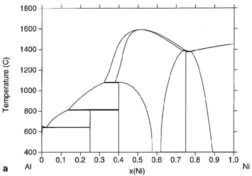
The progress that has been made with these reassessments is shown in Figure 2 for the Al-Ni system, a basic system for superalloys. In the first assessment of Kaufman and Nesor,47 the phases were either described as disordered solution phases [liquid, (Al), (Ni), and AlNi] or as stoichiometric compounds (Al3Ni, Al3Ni2, and AlNi3). The (Al) and (Ni) phases were described as one phase since they both have the fcc structure. Although the general topology of the experimentally determined phase diagram48 is reproduced, major differences occur for the equilibria involving the Al3Ni2 and AlNi phases. These differences are at least partially a result of ignoring the homogeneity range of the Al3Ni2 phase and not considering the fact that AlNi is an ordered phase with CsCl structure.
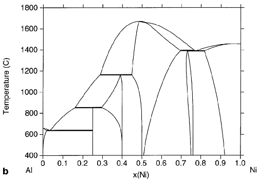
In the second assessment by Ansara et al.,38 the sublattice-model description was introduced for the ordered phases with noticeable homogeneity ranges (Al3Ni2, AlNi, and AlNi3). The disordered fcc phase [(Al) and (Ni)] and the ordered L12 phase (AlNi3) were described with a single free-energy function as one phase that undergoes an order/disorder transformation. While the phase diagram calculated from these improved analytical descriptions shows better agreement with the observed diagram, some noticeable disagreement still remains. The range of the (Al) solid solution is overestimated, and the region of single-phase AlNi3 slants to the nickel-rich side at lower temperatures. Both problems likely result from describing all of these phases with the single function. It should be also noted that the region of single-phase Al3Ni2 is overestimated at higher temperatures and underestimated at lower temperatures. This may be caused by the substitutional sublattice model description used in this assessment. It has been experimentally observed that on the nickel-rich side of the nominal stoichiometry, nickel atoms fill structural vacancies; on the aluminum-rich side, nickel atoms are substituted by aluminum.
This has been considered in the most recent assessment by Ansara et al.,39 who also modified the model for the description of the order/disorder transformation mentioned above. This assessment also includes a description of the Al3Ni5 phase as a stoichiometric compound, though its homogeneity range has been ignored. The phase diagram obtained from this assessment is in very good agreement with the observed diagram. It should be noted that the calculated phase diagram not only reproduces the experimentally observed phase diagram, but also provides the thermodynamic functions for extrapolation into higher order systems or use in the modeling of, for example, casting solidification.
A disadvantage of this iterative process with improved descriptions is that the descriptions used in previous assessments may be incompatible with newer assessments that are based on recently developed model descriptions. Despite this, significant progress has been made in recent years, and an increasing number of databases have become available for use with multicomponent systems.
The development of increasingly user-friendly computer interfaces, very often in conjunction with programs for special tasks, such as the ETTAN Windows interface54 for Thermo-Calc or the Scheil and Lever programs,55 makes phase-diagram information more accessible for the non-expert user. For these applications, the user needs only to supply a bulk composition and temperature limits for the calculation, and the programs generate the remaining conditions that are needed for the calculation.
For the incorporation of phase-equilibria calculations into micromodeling (e.g., the modeling of diffusion processes), an interface must be created in which the important variables are transferred from one computer code segment to another. For the simulation of diffusional reactions, Thermo-Calc51 has been interfaced with the package DICTRA.56 A general interface (TQ interface) is available for Thermo-Calc and ChemSage.57 Banerjee et al.28 used another, fairly simple interface for solidification micromodeling.
Several thermodynamic databases have been constructed from the assessments of binary, ternary, and quaternary systems. For the description of commercial alloys, it is quite likely that at least a dozen elements need to be considered. The number of constituent subsystems of an n-component system is determined by the binomial coefficient  , where k is the number of components in the subsystem. A 12 component system consists accordingly of 66 binary, 220 ternary, and 495 quaternary subsystems. These numbers suggest that is impossible to obtain descriptions of all the subsystems in reasonable time. However, as mentioned previously, only rarely are quaternary excess parameters needed. If the database is for base element X, it is sufficient to consider only the X-based ternary systems, hence, considerably reducing the number of needed assessments. Also, if more than one element occurs only in fairly small quantities in the alloy family of interest then assessments for binary systems containing only these elements or ternary systems with two or three of these elements are generally not very important for obtaining correct predictions.
Based on this information, databases have been developed for various commercial-alloy systems.58,59 However, because the software packages assume different computer file formats for the databases, care must be taken in order to insure compatibility between database and program package.
A review of fully integrated thermochemical database systems that were available in 1990 is provided by Bale and Eriksson.60 Since then, their review has been complemented by a site on the World Wide Web.61
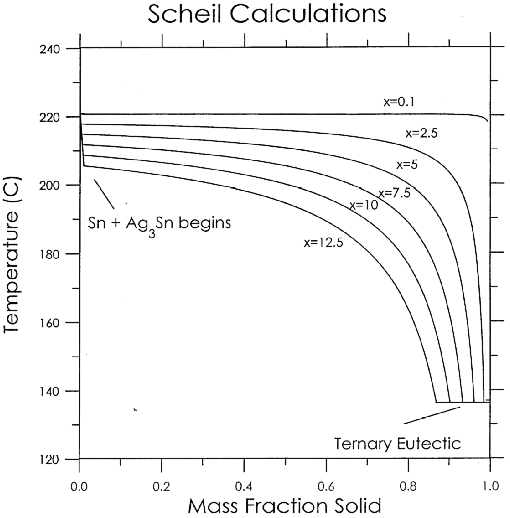
As mentioned, extrapolation to higher component systems is one of the staples of CALPHAD, since it provides information where otherwise only educated guesses could be used. When alloys of the Sn-Ag-Bi system were considered as candidate alloys for lead-free solders, no phase-diagram information for the liquid phase could be found. Kattner and Boettinger65 extrapolated the descriptions of the binary systems to calculate the solidus and liquidus surfaces of the tin-rich corner (Figure 3). The silver-rich side of the eutectic troughs should be avoided because the liquidus temperature increases significantly with increasing silver concentration. Figure 3 can be used to identify composition regimes where the freezing range is suitable for solder applications.
Two simple models describe the limiting cases of solidification behavior. First, complete diffusion is assumed in the solid as well as in the liquid for solidification obeying the Lever rule at each temperature during cooling. Thus, all phases are assumed to be in thermodynamic equilibrium at all temperatures during solidification. In comparison, solidification following the Scheil path, where diffusion in the solid is forbidden and thermodynamic equilibrium exists only as local equilibrium at the liquid/solid interface, produces worst-case microsegregation with the lowest final freezing temperature. Modeling of real solidification behavior requires a kinetic analysis of microsegregation and back diffusion; however, for most alloys, the predictions of the Scheil model are close to reality.
Scheil and Lever rule calculations were carried out for six alloy compositions in the solder alloy Ag-Bi-Sn system. The results are shown in Figure 4. The formation of eutectic due to segregation in the Scheil solidification increases the freezing range drastically. A comparison of Figure 4a and Figure 4b shows that as the equilibrium freezing range is increased (by adding bismuth), the Scheil solidification curve begins to deviate from that of the Lever rule solidification at smaller values of solid fraction formed. This is an indication that nonequilibrium solidification has a smaller impact on the actual freezing range of an alloy with a small equilibrium freezing range than an alloy with a large equilibrium freezing range. Because it is a practical requirement that solders should have a limited freezing range, this is important information for use in the design of new solder alloys.
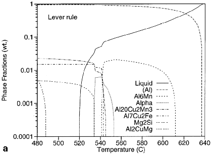
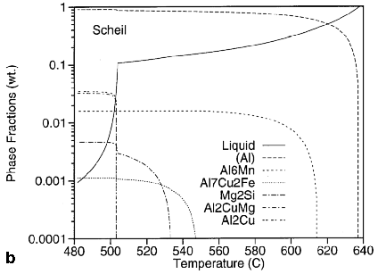
A phase-fraction diagram vs. temperature diagram is a very useful form of graphically presenting multicomponent alloys. Such diagrams are shown in Figure 5 for Lever rule and Scheil calculations of an alloy that is close in composition to the commercial aluminum alloy 243. The composition (in weight percent) used for this calculation is Al-4.44Cu-1.56Mg-0.55Mn-0.23Fe-0.21Si-0.05Zn. For the calculations, the Al-DATA database59,66 was used. The difference between Lever rule and Scheil solidification becomes most noticeable toward the end of solidification. For both solidification paths, the solidification begins with the precipitation of aluminum and Al6Mn. The Lever solidification, shown in Figure 5a, continues with the formation of the a-phase, Al20Cu2Mn3, Al7Cu2Fe, the decomposition of Al6Mn and the a-phase, and the formation of Mg2Si. Finally, after solidification is complete, precipitation of Al2CuMg begins. The final microstructure consists mainly of aluminum and small amounts of Al20Cu2Mn3, Al7Cu2Fe, Mg2Si, and Al2CuMg.
The Scheil solidification, shown in Figure 5b, continues with the formation of Al7Cu2Fe, Mg2Si, Al20Cu2Mn3 (this phase is not shown in the figure since the amount is extremely small), Al2CuMg, and Al2Cu. The microstructures obtained from these paths are quite different, which might result in different mechanical properties. The actual microstructure can be compared to diagrams like those shown in Figure 5, and casting parameters can be adjusted to obtain the desired microstructure by following a solidification path somewhere between these extremes.
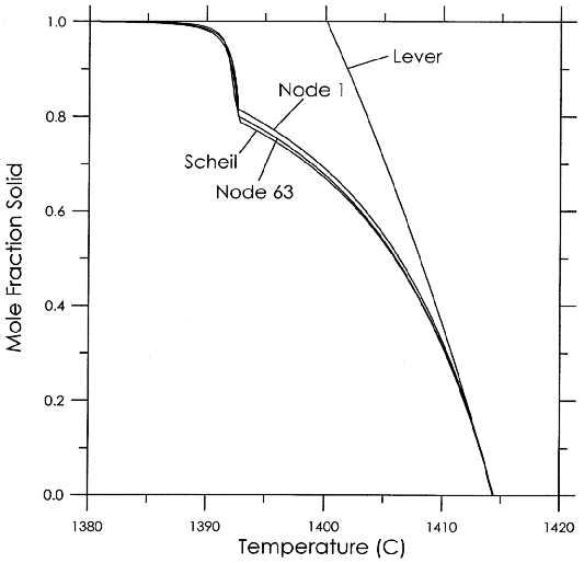
Major progress in the application of phase-diagram information has been made in the implementation of such calculations in casting simulation software. Thermodynamic calculation of the phase equilibria of a multicomponent alloy was interfaced with a micromodel for computing the change of fraction solid and temperature, given a specified change in enthalpy during the liquid-solid transformation. This coupling was incorporated into a finite-element package developed for modeling the solidification of castings. The simulation was carried out for a step wedge part and a Ni-15Al-2Ta (in weight percent) alloy. Further details of the simulation are described by Banerjee et al.28 Two nodes (points on the finite-element mesh) were selected to demonstrate the effect of the different cooling histories. One node (node 63) cooled approximately twice as fast as the other one (node 1). The fraction solid vs. local temperature curves were calculated for these two nodes during runtime and are compared to those of the limiting Scheil and Lever rule curves in Figure 6, with the curve of the slower cooling node revealing a slightly less pronounced Scheil behavior, and thus less segregation than the faster cooling node. These differences in Scheil behavior and segregation are expected to appear in the final casting and to be reflected in changing microstructure and properties varying throughout the casting.
For more information, contact U.R. Kattner, National Institute of Standards and Technology, Building 223, A153, Gaithersburg, Maryland 20899; e-mail ursula.kattner@nist.gov.
Direct questions about this or any other JOM page to jom@tms.org.
| Search | TMS Document Center | Subscriptions | Other Hypertext Articles | JOM | TMS OnLine |
|---|