This article is one of five papers on computer tools for materials to be presented exclusively on the web as part of the April 1997 JOM-e—the electronic supplement to JOM. The coverage was developed by Steven LeClair of the Materials Directorate, Wright Laboratory, Wright-Patterson Air Force Base. Please tell us know what you think by taking the survey below.
	The following article appears as part of JOM-e, 49 (4) (1997), http://www.tms.org/pubs/journals/JOM/9704/Gorni/ JOM is a publication of The Minerals, Metals & Materials Society

The Application of Neural Networks in the Modeling of Plate Rolling Processes

Neural networks are a relatively new artificial intelligence technique that emulate the behavior of biological neural systems in digital software or hardware. These networks can "learn," automatically, complex relationships among data. This feature makes the technique very useful in modeling processes for which mathematical modeling is difficult or impossible. The work described here outlines some examples of the application of neural networks in the modeling of plate mill processes at Companhia Siderúrgica Paulista, a Brazilian steelmaker.

INTRODUCTION

During the late 1980s, a revolutionary approach for data and information processing appeared—neural networks. This technique does not require the previous development of algorithms or rule sets to analyze data. This can significantly minimize the software-development work needed for a given application. In most cases, the neural network is previously submitted to a training step using known data; then the methodology necessary to perform the required data processing is extracted. Thus, a neural network is able to identify the required relationships from real data, avoiding the previous development of any model.

NEURAL NETWORKS: A TUTORIAL

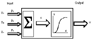Figure 1. A schematic representation of a neuron.

The basic element of a neural network is called, naturally, a neuron. It is also known as a node, processing element, or perceptron (Figure 1). The links between neurons are called synapses.

The input signal to a given neuron is calculated as follows. The outputs of the preceding neurons of the network (i.e., their state or activation values X₁, X₂, and X₃ in the specific example of Figure 1) are multiplied by their respective synapse weights, P₁, P₂, and P₃. These results are added, resulting in the value u that is delivered to the given neuron. By its turn, the state or activation value of this neuron is calculated by the application of a threshold function to its input value, resulting in the final value v. This threshold function, also called activation function, is frequently nonlinear and must be chosen critically, as the performance of the neural network heavily depends on it. Generally, this function is critically, sigmoidal.

How can a neural network learn? During the training step, real data (input and output) are continuously presented to it. It periodically compares real data with results calculated by the neuron network. The difference between real and calculated results (i.e., the error) is processed through a relatively complicated mathematical procedure, which adjusts the value of the synapse weights in order to minimize this error. This is an important feature of the neural networks; their knowledge is stored in their synapse weights.

The duration of the training step must not be excessively short so as to allow the network to fully extract the relationships between variables. Neither can this step be very long; in this case, the neural network will simply memorize the real data delivered to it, forgetting the relationships between them. So, it is advisable to break away approximately 20% of the available data in a subset and use only the remaining 80% for training the neural network. The training step must be interrupted periodically and the network tested using the 20% subset, checking the precision of the calculated results with real data. When the precision of the neural network stabilizes and stops to grow, it is time to consider the neural network fully trained.

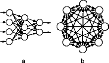Figure 2. The (a) Rummelhart and (b) Hopfield and types of neural networks.

Figure 2 shows two basic types of neural networks regarding data flow and training. The Rummelhart-type neural network (Figure 2a) shows data flow in one direction (i.e., it is a unidirectional network). Its simplicity and stability make it a natural choice for applications such as data analysis, classification, and interpolation. Consequently, it is particularly suitable for process modeling, and, in fact, there are many real-world applications of this type of network. A fundamental characteristic of this network is the arrangement of neurons in layers; such as, there must be at least two layers—data input and data output. As the performance of two-layer neural networks is very limited, it generally includes at least one more intermediate layer, also called the hidden layer. Each neuron is linked to all of the neurons of the neighboring layers, but there are no links between neurons of the same layer. The behavior of the Rummelhart network is static; its output is a reflection of its respective input. It must be previously trained using real data in order to perform adequately.

The Hopfield neural network (Figure 2b), on the other hand, has multidirectional data flow. Its behavior is dynamic and more complex than the Rummelhart network. The Hopfield networks do not show neuron layers; there is total integration between input and output data, as all neurons are linked between themselves. These networks are typically used for studies about the optimization of connections. This kind of neural network can be trained with or without supervision; the purpose of its training is the minimization of its energy, leading to independent behavior. However, there is no practical application for this network at this time.

Applications particularly suited for neural networks are those in which mathematical formulation is very hard or impossible. Some examples are signal analysis and processing, process control, robotics, data classification, data smoothing, pattern recognition, image analysis, speech analysis, medical diagnostics, stock market forecasting, analysis for loan or credit solicitations, and oriented marketing.

The comparison between neural networks and expert systems shows that the development of the former is faster, simpler, and cheaper. However, a major drawback to the use of neural networks arises from the fact that it is not always possible to know how a neural network obtained a given result. Sometimes, this can be very inconvenient, mainly when the neural-network-calculated results are atypical or unexpected. However, the use of hybrid artificial intelligent systems (e.g., conjugated use of neural networks with expert systems or fuzzy logic) are increasingly showing good results through the optimized use of its best characteristics.

There are some advantages of neural networks over multiple regression. There is no need to select the most important independent variables in the data set, as neural networks can automatically select them. The synapses associated with irrelevant variables readily show negligible weight values; on its turn, relevant variables present significant synapse weight values. There is also no need to propose a model function as required in multiple regression. The learning capability of neural networks allows them to discover more complex and subtle interactions between the independent variables, contributing to the development of a model with maximum precision. In addition, neural networks are intrinsically robust (i.e., they show more immunity to noise present in real data); this is an important factor in modeling industrial processes.

It must be noted that the use of statistical techniques can be extremely useful in the preliminary analysis of the raw data used to develop a neural network. Data can be refined, minimizing even more the development time and effort of a reliable neural network as well as maximizing its precision. Hybrid statistical-neural networks systems can be a very useful solution to some specific problems.

PLATE MILL APPLICATIONS

• The sizing of slabs for plate rolling.⁶
• The modeling of a steel's hot strength of steel based on temperature, strain, strain rate, and effect of chemical composition.^7,8
• The determination of TTT diagrams from the chemical composition of a steel.⁹
• Pass-schedule calculation for hot-strip mills.^10,11
• The feasibility of producing particular grades of at a particular steelworks.¹²

All neural networks developed were of the Rummelhart type, with one hidden layer, and trained by the retropropagation method. The networks included a bias neuron in the input layer to improve the modeling capacity of the neuron network.¹

In each case, 80% of the global raw data was reserved for training the network; the remaining 20% was periodically used during the precision evolution check of the neural network. The training step of most of the neural networks studied in this work converged in 60,000 iterations. Evaluation of the neural network was performed by calculating Pearson's correlation coefficient (r) and the standard error of estimate (SEE); dispersion plots were also used. The software used for developing and training the neural networks was NeuralWorks.

THERMAL PROFILE OF SLABS IN THE REHEATING FURNACE

A neural network model was developed to forecast the inner temperature of the slabs being reheated as a function of reheating time and superficial temperatures. This is a case with a relatively easy mathematical solution, and, thus, allowed a ready comparison between the performance of the neural network and the conventional numerical models. After several configuration trials, a neural network with three layers was designed. The input layer comprised three neurons: reheating time (min.), slab upper surface temperature (°C), and slab lower surface temperature (°C). The hidden layer contained 13 neurons, and the output layer consisted of ten neurons, each of which representing a point in the instrumented slab where the temperature was measured.

Varying the number of neurons in the hidden layer, as well the use of more than one hidden layer, did not improve the performance of the neural network, which had its best performance in forecasting the temperature in the mid-thickness of the slab (r = ~0.997; SEE = 26.5°C). The worst performance occurred near the lower surface of the slab (r = ~0.993; SEE = 36.6°C). Figure 3 shows dispersion plots of the real and calculated temperatures for both areas considered. The neural network's performance was considered adequate, as it was similar to previously developed mathematical models, which showed errors of ~30°C.

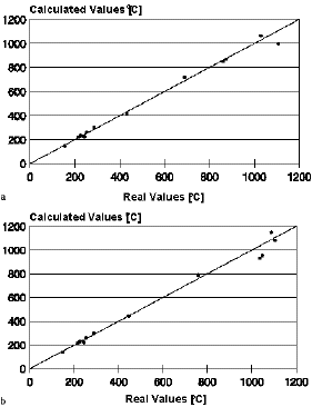Figure 3. Precision achieved by the neural network in modeling thermal profiles of a steel slab during reheating: (a) mid-thickness temperature; (b) near- the-lower-surface temperature.

DETECTING TURN-UP DURING PLATE ROLLING

Previous work showed that alterations in the pass schedule could minimize the occurrence of turn-up; this work led to the development of a statistical model for calculating an optimized pass schedule. There was a critical range of strain values to be avoided during plate rolling. However, this statistical model sometimes calculated unfeasible values of roll gaps. In some cases, the calculated values were excessively low, jeopardizing productivity; on other occasions, they were excessively high—well above the mill's capacity of load, torque, and power.

When neural networks became available, a natural application was to use them to address the problem of turn-up since the statistical model was unsatisfactory. After several trials, a neural network was developed consisting of an input layer with five neurons (i.e., desired turn-up index; work roll peripherical speed [rpm]; rolling load [t], calculated by the Sims model; rolling stock width [mm]; and roll-gap distance [mm] used in the former rolling pass). The hidden layer had eleven neurons, and the output layer contained one neuron, which represents the recommended roll gap distance (mm) for the next rolling pass.

The turn-up index used as an input variable was defined using an arbitrary scale from 0 to 5, representing porportional level of defect seriousness. The number of neurons in the hidden layer of this neural network was calculated after the Hecht-Kolmogorov's theorem, which affirms that the optimum number of neurons of a hidden layer is equal to twice the number of input neurons plus one.

The developed neural network showed r = 0.992 and SEE = ~3.0 mm. Figure 4 shows the dispersion plot of the real and calculated values. The most influential variables, as indicated by the trained neural network, are turn-up index and initial roll-gap distance, followed by (in a decreasing order of importance) rolling stock width, rolling load, and work-roll peripherical speed.

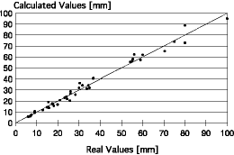Figure 4. Dispersion plot of the neural-network-calculated and real values for controling turn-up defects.

All calculated values are very near to the real values. That is, the neural network did not generate nonsense values as did the previously developed regression polynomial. Previous work about the turn-up occurrence at COSIPA's plate mill had revealed that this defect was more frequent in a specific range of roll-gap values: 60-80 mm. This is confirmed by the trained neural networks, as the initial roll-gap value is one of the most influencing variables of the model. In addition, the SEE is admissible, as it is equal to only 7.5% of the minimum roll-gap value. However, this is valid since the final thickness of plate is not between 40-80 mm.

LONGITUDINAL DISCARD CALCULATION WHEN USING PLANE-VIEW CONTROL

One potential solution to this problem is to apply a special thickness profile in the rolling stock during the application of the last pass of the broadsizing step. After this special pass, the width of the rolling stock presents a thickness profile that basically consists of a "V"-shape notch or the shape of a dog bone. The development of this process at COSIPA led to a 7% increase in the metallic yield of the plate mill.

During the development of this process, a regression polynomial was created to correlate the "V"-shape notch depth and the total strain applied to the rolled stock after the broadsizing step with the length of the discarded portion of the final rolled stock, thereby enabling a better understanding of the process and a check of its optimization possibilities. This polynomial presented r = 0.903 and SEE = 132 mm.

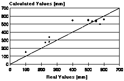Figure 5. Dispersion plot of the neural-network-calculated and real values for estimating the length of the discarded portion in plates submitted to plane-view control during rolling.

Once more, this appeared to be a good application for a neural network, as it could be an opportunity to improve the forecasting of the length of the discarded portion. The best neural network designed to substitute the polynomial equation had an input layer with two neurons ("V"-shape notch depth [mm] and total strain applied to the rolled stock after broadsizing step [%]); a hidden layer with five neurons (according to the already mentioned Hecht-Kolmogorov's theorem); and an output layer with one neuron (representing the length of the discarded portion in the final rolled stock [mm]). The neural network showed r = 0.943 and SEE = 61 mm. The dispersion plot of real and calculated values for the length of the discarded portion in the final rolled stock can be seen in Figure 5.

Although the neural network showed better performance than the regression polynomial (the SEE fell approximately 54%), errors observed in Figure 5 are still significant. Perhaps the cause of these relatively high errors stems from the use of the discard length as an evaluation parameter of the metallic yield of the process. This parameter is less representative than the weight or area of the discarded portion but, in compensation, is an easier variable to measure under industrial conditions.

PASS SCHEDULE CALCULATION

Figure 6. Dispersion plots for the pass schedule on optimizing plate flatness from the neural-network-calculated and real values of the roll gap for (a) the third to last, (b) of next to last, and (c) the last plate rolling passes.

Mathematical models for calculating pass schedules are relatively easy to develop, but the use of neural networks is simpler. The three last passes of the rolling schedule were modeled regarding optimization of plate flatness; one neural network was attributed for each pass. The three neural networks showed the same configuration. The input layer consisted of ten neurons (thickness of final plate [mm], width of final plate [mm], aimed flatness index in final plate, flatness index observed after prior pass, roll gap of prior pass [mm], rolling load measured during prior pass [t], temperature measured during prior pass [°C], original crown of the upper work roll [mm], original crown of the lower work roll [mm], and rolling stock tonnage since the last change of the work rolls [t]). The hidden layer had 21 neurons (according to Hecht-Kolmogorov's theorem), and the output layer had one neuron, which represents the roll-gap value of the corresponding pass (mm).

The flatness index used in this model varied from 0 to 5 (the higher the number, the worse the plate flatness). The performance of the neural network was very good. Corresponding to the last three passes, r = 0.998, 0.998, and 0.999, respectively; SEE = 0.430 mm, 0.394 mm, and 0.140 mm, respectively. Figure 6 shows the dispersion plots of the real and calculated values for the final three passes of the rolling schedule.

The most important variables in these neural networks were the aimed flatness index, the original crown in the upper work roll, and the rolling-stock tonnage after the last change of work rolls. There were also parameters of intermediate importance, such as the final plate width/thickness and temperature/load of the prior pass. Finally, variables like prior pass flatness index/roll gap did not show great influence, but were vital to improving the precision of the neural networks, making its use feasible under industrial conditions.

In fact, during the learning step, the neural networks identified the most important variables related to flatness that are traditionally defined by the rolling theory—original crown of work rolls and rolling-stock tonnage since a change of work rolls. This last variable generally shows good correlation with thermal crown and wear of work rolls—factors that affect the resultant roll crown and, consequently, plate flatness. Work roll deflection promoted by rolling load was also considered, as this was included in the input layer of the neural networks.

The last pass is the most important to define the final dimensions of plate, especially its thickness. The errors observed in the results calculated by the respective neural networks varied from -0.26 mm to +0.17 mm—practically within the commercial-plate-thickness tolerance range. The results can be further improved as more precise data acquisition systems become available. Such systems would avoid human error during data collection and improve the precision of the measured parameters.

CONCLUSIONS

Unfortunately, the lack of instrumentation, data acquisition capabilities, and computer facilities at COSIPA's plate mill hindered the on-line application of these models. One of the disadvantages of neural networks is the complexity of hardware and software necessary to enable industrial application. For example, if process conditions change from those used when training the neural network, data must once again be collected, analyzed, and used for retraining the system.

Another issue to consider is the lack of confidence some people feel about the performance of the neural networks, as it is difficult to understand how, exactly, these networks generate results. This reservation with the technology will be corrected in time, however, as the application of neural networks becomes more commonplace and the reliability of their results is demonstrated.

References

For more information, contact A.A. Gorni, Rua Joáo Ramalho 315/103, 11310-050, Sao Vincente, Sao Paulo, Brazil; telephone 5513 467-1805; fax 5513 362-3608; e-mail agorni@dialdata.com.br.

Will You Take a Short Survey?

References

1. R. Hecht-Nielsen, Neurocomputing, (Reading, PA: Addison-Wesley Publishing Company, 1990), p. 433
2. R.C. Eberhart and R.W. Dobbins, eds., Neural Network PC Tools—A Practical Guide (San Diego, CA, Academic Press, 1990), p. 414
3. B. Müller et al., Neural Networks: An Introduction (Berlin: Springer-Verlag, 1995), p. 330
4. J.A. Freeman, and D.M. Skapura, Neural Networks: Algorithms, Applications and Programming Techniques (Reading, PA: Addison-Wesley Publishing Company, 1992), p. 401
5. A. Blum, Neural Networks in C++ (New York: John Wiley & Sons, 1992), p. 214
6. J.B. Oliveira et al., "Use of Neural Networks in the Plate Production Scheduling at USIMINAS," Seminário de Laminação (Porto Alegre: Associação Brasileira de Metais, 1992), pp. 319-339.
7. A.A. Gorni, "Mathematical Modeling of the Hot Strength of HSLA Steels," 1st Metal Forming Week (Joinville: Associação Brasileira de Metalurgia e Materiais, 1993), pp. 267-286
8. J.G. Lenard et al., "A Comparative Study of Artificial Neural Networks for the Prediction of HSLA and Carbon Steels," Steel Research (February 1996), pp. 59-65
9. C. Dounadille et al., "Usage de Reseaux Neuronaux por Prevision des Courbes de Transformations de Acier," Revue de Metallurgie-CIT (Oct. 1992), pp. 892-894.
10. B. Ortmann et al., "Modernization of the Automation in the Hot Wide Strip Mill at Voest-Alpine Stahl," Metallurgical Plant and Technology-International (6) (1994), pp. 26-34.
11. N. Portmann et al., "Application of Neural Networks in Rolling Mill Automation," Iron and Steel Engineer (2) (1995), pp. 33-36.
12. M. Watanabe et al., Development of Shape Steel Quality Design Expert System, Nippon Steel Technical Report (April 1992), pp. 29-44.