TMS ONLINE | TMS PUBLICATIONS | SITE MAP An Article from the December 2003 JOM-e: A Web-Only Supplement to JOM

VISIT THE JOM COVER GALLERY JOM MENU

INTRODUCTION

Students majoring in materials science and engineering at Pennsylvania State University take a course that addresses transport phenomena in materials processing, including extended coverage of diffusion in solids. To assist in teaching this subject, the authors have created two pieces of software for use during the portions of the course covering heat transfer and diffusion. The first program allows us to introduce students to computer solutions for heat transfer and diffusion problems. In some cases, we wanted students to tackle problems numerically that they could not handle analytically. In others, we simply wished to provide an opportunity for the students to better visualize solutions. We did not want to encumber students with too much programming, since only one semester is devoted in our curriculum to fluid flow, heat transfer, and diffusion in materials processing. The new MATLAB toolbox we developed called FDPDE allows us to simultaneously achieve these goals. We have also created a program called Random Walk to assist students in understanding the atomic mechanisms of diffusion.

A NEW MATLAB TOOLBOX: FDPDE

Our new toolbox for MATLAB called FDPDE allows students to solve either steady-state or time-dependent heat transfer and diffusion problems in two dimensions using the finite-difference approach. Use of the toolbox requires that the commercially available program MATLAB be installed, but minimal working knowledge of MATLAB is actually needed to use the toolbox. (See sidebar for details on how to obtain the software.)

Before using the software, we briefly introduce students to the finite-difference approach so that they have an understanding of the method used by the toolbox to solve partial differential equations. A simple introduction to the technique can be found in Gaskell’s text on transport phenomena in materials engineering.¹ More details about the solver are provided in the user’s manual, which can be downloaded from our web site at www.esm.psu.edu/matls-sim/. The user's manual also explains in detail how to use the program. In this article, we only briefly illustrate some of the capabilities of the software, describing how it can be used to solve an example problem adapted from Poirier and Geiger’s text:²

Polypropylene is injected at 500 K into a mold to form a long strip that is 4 mm thick and 10 mm wide. The resistance to heat transfer at the interface between the plastic and the metal mold is negligible, as is the resistance to heat transfer within the metal mold, so the surface of the polymer quickly reaches the temperature of the mold (300 K) and remains there. The plastic may not be ejected until the center line is 360 K. Calculate the time required before the plastic can be ejected (calculate the “freeze-off” time). For polypropylene, use r = 900 kg/m3, Cp = 1900 J/kg•K, and k = 0.12 W/m•K.

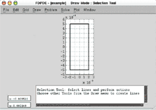
To begin, the student chooses to solve a heat transfer rather than diffusion problem using the Problem menu. Next, he or she pulls down the Draw menu and goes into Draw mode, as shown in Figure 1. The student creates a rectangle with the proper dimensions, which is the cross section of the plastic strip in this problem. For other problems, more complicated shapes can be constructed from line segments and portions of rectangles and ellipses.

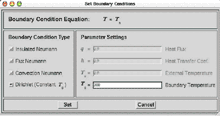
Figure 1. A cross section created in Draw mode.		Figure 2. The Set Boundary Conditions dialog box.

In the example problem, the condition on the boundary is a constant temperature (300 K). The boundary is selected, and from the Problem menu, the Set Boundary Conditions dialog box is brought up, as shown in Figure 2. In other problems, several types of boundary conditions may be appropriate along different portions of a cross section, and the boundary can be divided into segments so that different boundary conditions can be applied to each segment.

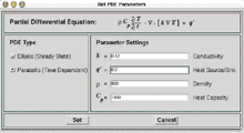
Next, the rectangle is again selected, and from the Problem menu, a domain is created. When the domain is created, a dialog box automatically appears that allows the student to set the parameters for the equation that apply to this problem. Since this is a time-dependent problem, he or she chooses the parabolic partial differential equation

where r is the density, C_p is the specific heat, T is temperature, t is time, k is thermal conductivity, and is the rate of heat generation (zero in this problem). The properties of the material, such as density, specific heat, and thermal conductivity (in consistent units) are then entered, as shown in Figure 3.

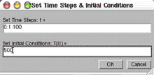
Figure 3. The Set PDE Parameters dialog box.		Figure 4. The dialog box for time steps, total integration time, and initial conditions.

The next step is to solve the differential equation. Working from the Solve menu, the student selects the number of nodes to be used in the solution. In this example, we have chosen 17 x 41 nodes. Since this example problem includes time as a variable, the student must also enter an initial condition and select time steps as well as the total length of time over which the equation is to be integrated. As shown in Figure 4, an initial temperature of 500 K and 100 time steps of 1 s each are chosen.

It is important for the students to understand that their solutions become inaccurate if the nodes are spaced too far apart or the time steps are too large. On the other hand, it takes a very long time for the computer to solve a problem if the nodes are too close together or time steps too short. Having the students systematically adjust the node spacing and time steps and evaluate the results helps them recognize this tradeoff.

Once the problem is solved, students have several options in the Plot menu. They may plot the temperature distribution across the cross section at a given time, view the temperature distribution across the cross section as it changes with time by generating a movie, or plot the temperature as a function of time at one or more points within the cross section. Two such plots for our example problem are provided. In Figure 5, we see the temperature distribution across the cross section at 5 s. In Figure 6, we see the temperature as a function of time at the center of the strip, which allows us to determine that the center of the strip reaches 360 K after about 33 s.

Figure 5. The temperature distribution after 5 s in the rectangle described in the example.		Figure 6. The temperature as a function of time at the center line in the rectangle described in the example.

Student response to the software was favorable. When asked through an anonymous survey if they found the software easy to use, 80% of the students in a class of 25 answered “yes.” Only 12% answered “no,” while 8% said the software was somewhat easy to use. Interestingly, 8% also commented that they would probably have found the software easier to use had they come to class the day it was introduced. In response to the question, “Did the software help you better visualize the solutions to heat transfer problems?” 92% of the class answered “yes,” 8% answered that the software “somewhat” helped, while no student said it was not helpful.

We received some interesting responses to the question, “Did the software help you better understand how to solve heat transfer problems?” A majority of students (56%) answered “yes,” and some of the students elaborated on how the program was helpful. One student replied, “It made me think about the problem instead of just inputting data.” Another said, “The problems done in class and in HW are so rigid . . . With the software I can see other events happening and not just what the problem is focused on.” Another student indicated that he or she could now “understand more clearly what steady state actually means.”

On the other hand, we were initially disappointed that 8% of the class responded that the software had only “somewhat” helped them understand how to solve heat transfer problems, while 36% said it had not helped. However, some of the explanations for why the software did not help illustrated that the software was actually performing much as we had intended. For example, one student who did not find the software helpful noted, “You need to understand what you wanted to do in order for the software to be useful.” Of course, we had intended to require students to recognize which differential equation needed to be solved and which variables were important in their problems. The purpose of the software was to help them easily solve the equations and visualize the solutions. Another student remarked, “Once the variables were identified, it was easy to just plug your way through a problem.” Since we had not intended for the software itself to be difficult to use, we also did not consider this comment to be entirely negative.

THE RANDOM WALK PROGRAM

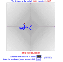
As an aid to teaching about diffusion, a second program called Random Walk was created to illustrate the outcome of many random walks by either one or many atoms. The programming for this piece of software was performed by Kunal Ruvala and Gautam Sarda using Macromedia Director. The Random Walk program is a stand-alone application and is also available free of charge through our web site.

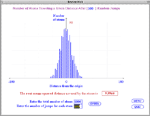
Figure 7. The output for two-dimensional random walk.		Figure 8. The output for one-dimensional random walk.

The software provides two modes of operation. First, it can be used to animate a random walk by one atom on a two-dimensional plane, providing output similar to that of Figure 7. Alternatively, it can be used to generate a histogram for a large number of atoms after each atom has randomly jumped to the left or right a given number of times. A screenshot of this part of the program is shown in Figure 8. One way this program can be used is to ask students to collect data for the root-mean-square (RMS) distance traveled for different numbers of total jumps, and then ask them to use Microsoft Excel (or a similar program) to fit an equation to their data. They discover on their own that the RMS distance traveled is proportional to the square root of the number of jumps. This software has already been successfully been used at Penn State.

ACKNOWLEDGEMENTS

The authors wish to acknowledge support from the National Science Foundation through DUE 9952597 and the Penn State Materials Research Institute.

References

1. David R. Gaskell, Introduction to Transport Phenomena in Materials Engineering (New York, NY: Macmillan Publishing Company, 1992).
2. D.R. Poirier and G.H. Geiger, Transport Phenomena in Materials Processing (Warrendale, PA: TMS, 1994).

For more information, contact Suzanne Mohney, Pennsylvania State University, Department of Materials Science and Engineering, 109 Steidle Building, University Park, Pennsylvania 16802; (814)863-0744; fax (814)865-2917; e-mail mohney@ems.psu.edu.