|
Empirical Potentials for Concentrated Alloys
|
An elementary treatment of alloys that nonetheless preserves much of their complexity
is based on the quasi-chemical expression for the energetics of an ensemble of atoms (see
Equation 1), where φi,j Ε {φAA, φAB, φBB} represents the contribution to the total energy
of a bond between atom types AA, AB, or BB, in a binary alloy of A and B species. (All
equations appear in the table.) In a random solid solution of composition xB,
with xA+xB = 1, where atoms have coordination z, the total energy per atom is given in
Equation 2, with Ω = φAB{(φAA+φBB)/2}. Ω measures the departure of the heteroatomic
interaction from the average interaction between the species. The heat of formation (h.o.f.)
of the alloy (i.e., the departure of the energy of the alloy with respect to the ideal solution;
ideal solution energy is given by the linear interpolation between the pure constituents) is
simply given by Equation 3.
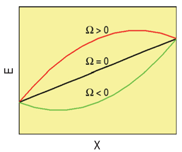
In this model then, the h.o.f., Δef, is a quadratic (symmetric) function of composition,
with Ω > 0 for solutions showing a tendency to segregate and Ω < 0 for those with tendency
to form compounds. Figure A shows the energy of the solution versus composition for the
three possible cases.
Many solutions in nature do not have a symmetrical h.o.f. and therefore additional
complexity is usually added to this elementary treatment by introducing a polynomial
dependence of Ω on composition, usually called sub-regular solution model, using a
particular form called the RedlichKister expansion, as shown in Equation 4, where Lp
are coefficients dependent on temperature. Empirical potentials for molecular dynamics
(MD) simulations of alloys are built upon expressions similar to the quasi-chemical
energetics, but with radial dependence and non-linear terms. The many-body potentials
have in common a description of the total energy in terms of the sum over atom energies,
themselves composed of two contributions, namely embedding and pair potential terms;
it reads as shown in Equation 5, where α and β stand for elements A or B sitting at sites i
or j; Fs are the embedding functions for either type of elements, and Vs and ρs are the pair
potentials and densities between αβ pairs. Alloy properties are therefore described by
the functions ρAB and VAB. Depending on the model considered, the density functions do
not always include the cross term ρAB. Different expressions for the embedding energies,
densities, and pair potentials englobe a large diversity of similar models.
From Equation 5 it appears clearly that the h.o.f. of such an alloy has contributions
from the non-linear embedding term and from the pair potential functions. The latter
provide a contribution to the h.o.f. equivalent to the Ω term in Equation 2. In order to
reproduce complex formation energies, a natural way to add complexity into the model,
as suggested by Equation 4, is to include a composition dependence to the pair potential.
The composition is a local variable, depending on the environment around atoms i and j
(a detailed derivation is given in Reference 9). See Equations 6 and 7.
For h(xi,j) a representation was chosen based on the RedlichKister expansion of
the same order n used to fit the h.o.f one wants to model, namely Equation 8, with Hp
coefficients obtained by a fitting procedure. This procedure proves robust in the sense
that given a target h.o.f. is always possible to find an embedded atom type model as
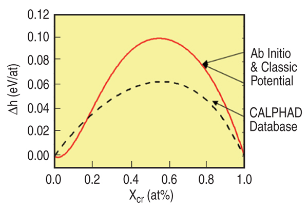
given by Equation 6 that reproduces it. Figure B shows the results for FeCr with the
target h.o.f taken from the ab-initio calculations of Olsson et al.10 The formation energy is
indistinguishable from the target function.
FROM POTENTIALS TO THERMOSYNAMICS
The calculation of the thermodynamic properties of an alloy implies the knowledge of
the free energy of the different phases as a function of composition and temperature. The
calculation of the free energy is a multi-step process that requires several different MD
runs. In recent papers, a numerical package was implemented that allows efficient and
accurate calculation of free energy. A complete description of the method is available in those previous publications.1113The basic assumption that links thermodynamics
to MD is ergodicity represented by the assumption
in Equation 9, where the left-hand side is a time
average in an MD run, namely Equation 10, and
the right-hand side is an ensemble average in the sense of statistical mechanics (see Equation 11, where H is the Hamiltonian of the system, ξ is the ensemble of variables that specify a particular state, k is the Boltzman constant, T
is the temperature, and Ω is the volume of the phase space).
Free energy is not an ensemble average, it is rather related to the denominator of
Equation 11 (see Equation 12) and cannot therefore be obtained as a time average of
an MD run. Numerous procedures to calculate free energies have been proposed and
are available for review in the literature. 1419 Here, the free energy per particle at a given
temperature T, F(T), is calculated through a thermodynamic integration between the state
of interest and a reference state at temperature T0 with known free energy F(T0), using the
Gibbs-Duhem equation, as shown in Equation 13, where h(t) is the enthalpy per particle.
The enthalpy is obtained from an MD run and it is fitted with a polynomial in T that
allows an analytic integration in Equation 13. The coupling-constant integration method,
or switching Hamiltonian method, is used to calculate F(T0). Considered here is a system
with Hamiltonian, as shown in Equation 14, where U represents the actual system (in
this work, described with a EAM-type Hamiltonian) and W is the Hamiltonian of the
reference system, with known free energy. The parameter λ allows the switch from U (for
λ = 1) to W (for λ = 0). With this Hamiltonian one can obtain the free energy difference
between W and U by calculating the reversible work required to switch from one system
to the other. Then the unknown free energy associated with U, F(T0), is given by Equation
15, where FW(T0) is the free energy of the reference system at T0. The integration is
carried over the coupling parameter λ, and <
> stands for the average over a canonical
ensemble, or a time average in a (T, V, N) constant MD simulation. For the solid phases
the reference system W is a set of Einstein oscillators centered on the average positions
of the atoms in the (T, P = 0, N) ensemble corresponding to the Hamiltonian U. The free
energy per atom of the Einstein crystal is known analytically and therefore Equations 13
and 15 provide the recipe for free energy calculations.
For alloys the strategy is to construct for each phase of interest a set of free energy
functions versus composition x and temperature F(x,T).
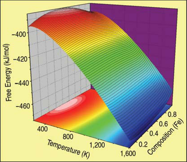
The final result for the free energy of the FeCr alloy in the body centered cubic
ferromagnetic phase is shown as a surface in Figure C. Isotherm lines, in black over the
surface, are used together with the common tangent construction to determine the phase
diagram shown in Figure 4.
|
This paper describes a strategy to
simulate radiation damage in FeCr alloys
wherein magnetism introduces an
anomaly in the heat of formation of the solid solution. This has implications for
the precipitation of excess chromium in
the a' phase in the presence of heterogeneities.
These complexities pose many
challenges for atomistic (empirical)
methods. To address such issues the
authors have developed a modified manybody
potential by rigorously fitting
thermodynamic properties including free
energy. Multi-million atom displacement
Monte Carlo simulations in the transmutation
ensemble, using the new potential, predict that thermodynamically
grain boundaries, dislocations, and free
surfaces are not preferential sites for α′
precipitation.
INTRODUCTION
The accurate prediction of innumerable
properties of the many diverse
materials, comprising multiple constituents
as well as time and space scales, is
nowadays considered routine. This
quantitative computational materials science relies on a combination of quantum
mechanics and thermodynamics/
statistical mechanics. These two pillars
complement each other well. While
quantum mechanics, especially density
functional theory (DFT),1 provides the
basis for an almost parameter-free theory
for the potential energy landscape, statistical
ensemble sampling using numerous
approximations allows various
thermodynamic properties to be estimated.
2
Many problems, frequently related to
non-equilibrium properties, cannot be
addressed directly by the state-of-the-art
ab-initio approach; approximations have
to be used. Progress in computational
capabilities and algorithm efficiency will
not overcome these limitations in the
foreseeable future. For that reason simplified
models for the energetics are
customarily used to capture partial
aspects of reality, furthering the understanding
of complex physical processes.
For example, classical potentials are
widely used for large-scale dynamic
simulations of a diversity of systems, in
particular, metals.35 At present such
potentials show much promise for
describing basic thermodynamic properties
of complex, multicomponent materials.
When mechanical properties and
microstructure are the focus of attention,
simulations have to be simple enough to
deal with a large number of atoms, thus
capturing the length scale that is relevant
for this class of problems. The classical empirical total energy expressions that
are so widely used have limitations to
address real materials. In particular, iron
alloys, the most commonly used materials
for structural applications, continue
to be a major challenge, as iron is a
complex element whose properties are
determined by subtle features in its
electronic structure. Furthermore, impurities,
intrinsic defects, and alloying
elements in iron play significant roles in
determining its macroscopic mechanical
properties. In nuclear reactors, structural
components and fuel cladding undergo
embrittlement as a consequence of
radiation-induced α′ precipitation. The
ability to perform predictive atomistic
simulations for alloys in such an environment
has attracted much attention.
FeCr alloys are common structural
materials in present fission reactors.
Their resistance to swelling, low ductile-to-brittle transition temperature, and low
activation properties make them good
candidates for use in future fusion reactors.6,7 High-energy particle bombardment
will extensively damage the alloy.
The displacement per atom (dpa) dose
expected in fusion reactors is in the range
of 100,8 inducing microstructure evolution,
swelling, and embrittlement.
FeCr ALLOYS IN IRRADIATION ENVIRONMENT
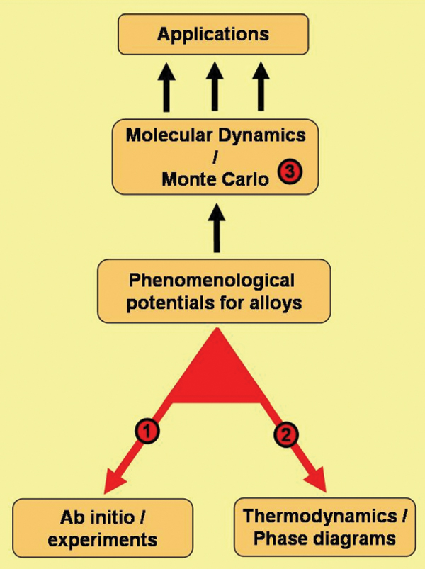
In the schematic shown in Figure 1, the
link labeled 1 shows the methodology
to utilize data obtained from ab-initio
calculations or experiments to formulate
empirical interatomic potentials appropriate
for large-scale molecular dynamics
(MD) simulations. To develop a potential
that reproduces variables relevant to the
problem of interest, properties such as
heat of formation (h.o.f.) of the alloys in
the entire compositional range, the lattice
parameter, or the elastic properties versus
composition are used. An overview of
the procedure can be found in the sidebar, and References 14 and 15
give details.
The calculation of the thermodynamic
properties of an alloy implies knowledge
of the free energy of the relevant phases
as a function of composition and temperature
(see link 2 in Figure 1). The free
energy calculation involves a multi-step
process requiring many MD runs. A
numerical package was implemented to efficiently and accurately calculate
free energies. A detailed description of
the method is available in References 14
through 18. See the Equations table for
the main equations.
Following the methodology proposed
in CALPHAD,11 the problem of binary
alloys was separated into the properties
of the pure elements (i.e., the free energies
of all possible phases of the pure
elements) and the properties of the mixtures.
The latter are expressed in terms
of excess enthalpy and entropy. Excess
quantities are referred to the linear interpolation
between the pure elements,
which represents the ideal solution. Now
the alloy description is conveniently
separated into two distinct parts: the
description of the pure elements and the
description of the mixture. Once the free
energies are expressed in this way (suggested
by the Scientific Group Thermodata
Europe)12 the calculation of phase
diagrams can easily be performed with
software such as Thermo-Calc.11
The numerical results can be compared
with a standard thermodynamic database
such as the Dinsdales compilation.13
Note that not all data in the database are
from experiments.
This work used the iron potential
reported by M.I. Mendelev et al.20 and
the chromium potential reported by J.
Wallenius et al.21 The formation energy
for FeCr has recently been calculated by
P. Olsson et al.10 together with a rough
estimate of the bulk modulus and lattice
parameter of the alloy as a function of
composition. These calculations, albeit
ab-initio, still contain several simplifications
and are therefore not to be considered
as definitive. They are first estimates
on which classical models can be developed.
T.P.C. Klaver et al.22 used DFT calculations
to study the mixing behavior of
FeCr alloys. They confirm the previous
observations by P. Olsson et al.10 and by
A.A. Mirzoev et al.23 regarding the
change in sign in the formation energy
of the alloy at x ~ 0.1 (where x refers to
chromium composition). The subtle
electronic structure that arises when
ferromagnetic (fm) and antiferromagnetic
(afm) metals are mixed in different
ratios appears to cause this anomaly. In
fact, magnetic frustration leads to a
strong dependence of the chromium
magnetic moment on the number of
chromium neighbors. Magnetic frustration
occurs when it is impossible for an
iron or a chromium atom to assume an
fm or afm state respectively, with respect
to all its neighbors. This translates into
a repulsive interaction that competes
with the large negative heat of solution
of a single chromium impurity (i.e., a
tendency to form ordered compounds).
The limitations of the quasi-chemical
description for the energetics of this
system (see the sidebar) become readily
apparent when we realize that in an
expression like Equation 1 the Cr-Cr
interaction has to be attractive since
chromium is in a condensed phase at 0
K, while it becomes repulsive when the Cr-Cr pair is surrounded by iron. It
implies then that a pair-like model for
the energetics has to contain explicit
composition-dependent terms.
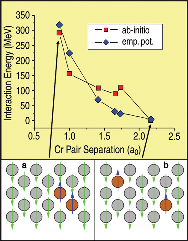
A first test of the approach is a comparison
of classical and ab-initio calculations
of the Cr-Cr interaction when a
chromium substitutional pair is embedded
in an otherwise pure iron matrix and
their separation distance is increased
(Figure 2). Apart from the fine structure
of the ab-initio results at the fifth-neighbor
separation, attributed to finite size
effects,22 the agreement in both strength
(~300 meV) and range (~2.2 a0) of the
interaction is very good, giving support
to this classical model as being able to
capture the Cr-Cr pair repulsion aspects
of the energetics in this system.
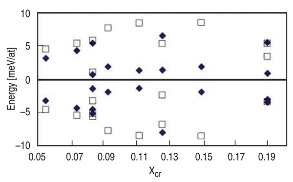
A more stringent test of the potential
is to compare the energy dispersion
between different configurations of
chromium substitutions at a given global
composition and sample size. Because
ab-initio calculations involve small
supercells, disordered configurations
always represent ordered supercell
structures with image interactions translating
into significant dispersion of the
results. On the other hand, simulations
based on empirical potentials can afford
large system sizes and thus many possible
local configurations of random
solutions are adequately explored, which
translates into small energy dispersion
between different realizations of the
random samples. It should be noted here
that the ab-initio results by Olsson10 used
by the authors to derive classical potential
do not have dispersion because they
are obtained using the coherent potential
approximation, a mean field methodology
for disordered alloys.
The ab-initio data that will be compared
with classical results were obtained
in supercells of 16, 24, and 54 atoms.
These numbers are too small for the
embedded atom model (EAM) formalism
(minimum size is twice the cutoff
of the interactions, involving ~100
atoms). The authors replicated the ab-initio
54 atom sample 3 × 3 × 3 times to
get the classical 1,458 atom sample, and
4 × 4 × 4 times for the smaller ones.
While this procedure reproduces some
of the finite size constraints appearing
in the ab-initio calculations, it still allows
for relaxations with wavelengths equal
to three or four times the size of the ab-initio supercell, not accounted for in the
ab-initio calculations; some discrepancies
are therefore expected. Finally, since
the classical potential is fitted to the h.o.f. by Olsson, and the results by Klaver
use a different ab-initio approach, the
comparison is done not in absolute values
but in dispersion around a mean. Figure 3
shows several cases, at different compositions
and cell sizes. The agreement in
the range of the dispersion between different
configurations goes from surprisingly
good in some cases to reasonably
good in others, within the accuracy of
the calculations. From Figures 2 and 3
one can conclude that the complexity of
the interactions in the solid solution is
reasonably represented by the classical
potential.
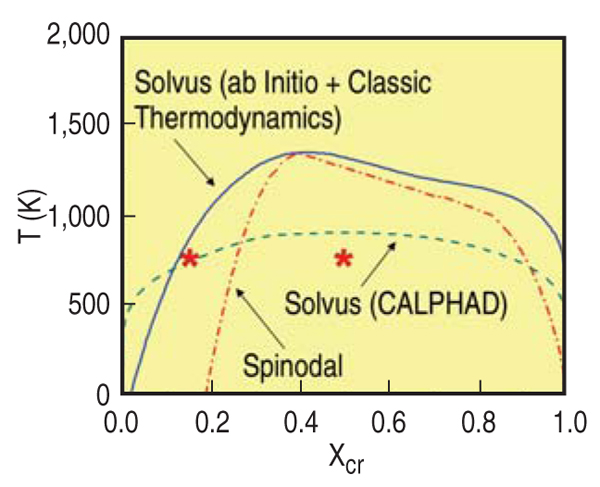
THERMODYNAMIC PROPERTIES
From the free energy function represented
in Figure C in the sidebar, the
miscibility gap and the spinodal are
obtained (Figure 4). For comparison,
this figure also shows the solvus as it
appears in SSOL, the database of
CALPHAD;11 note that all other phases
have been omitted. Several differences
are readily noticeable. Neither the miscibility
gap nor the spinodal go to zero
composition at 0 K on the iron-rich side
of the diagram. This curious effect is due
to the change in the sign of the h.o.f. of
this alloy at about 10%, which implies
finite solubility at low temperatures.
Additionally, the critical temperature for
this ab-initio plus classical thermodynamics
model is much higher (~1,300
K) than the value in the SSOL data. The
reason is that the h.o.f. data of Olsson,10
on which the potential is based, show a
maximum of about 100 meV, a value
well above the SSOL data (60 meV); on
the other hand, excess vibrational entropies
agree very well and contribute
significantly to the excess free energy.
For details see Reference 15.
To describe non-equilibrium processes
in heterogeneous systems with defects
and external potentials, a new computational
tool is needed. Most computational
approaches to non-equilibrium are based
on kinetic Monte Carlo (MC) algorithms
that in one way or another have to adopt
a frozen backbone or lattice where the
diffusing species jump. This is a necessary
restriction because a time-tracking algorithm needs rates for all possible
events.24
Kinetics and thermodynamics are two
aspects of the problem of evolution in
non-equilibrium systems.25 Since one
cannot yet treat both at the same level
of accuracy, one has to choose which
one is more relevant for the problem
under consideration. The focus here is
on thermodynamics, with a parallel MC
code that drives the system toward thermodynamic
equilibrium by minimizing
the free energy as MC steps go on, with
no approximations to the potential energy
landscape.
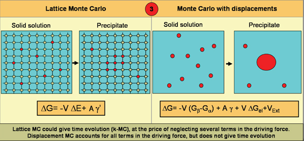
Figure 5 shows a schematic representation
of this algorithm. Details will be
published elsewhere.24 While the driving
force for a lattice algorithm is the difference
in energy between the two phases
plus a contribution from a simplified
interface energy, the displacements
algorithm accounts for all terms with no
approximations. Differences are seen in
free energy between the phases, actual
interfacial free energy, the contribution
from elastic energy created by lattice
mismatch, and interaction with external
potentials (external or internal stress
fields, originating in defects like grain
boundaries, cracks, dislocations, surfaces, etc). [VIEW ANIMATION to see an example
of the application to copper
impurities in iron.]
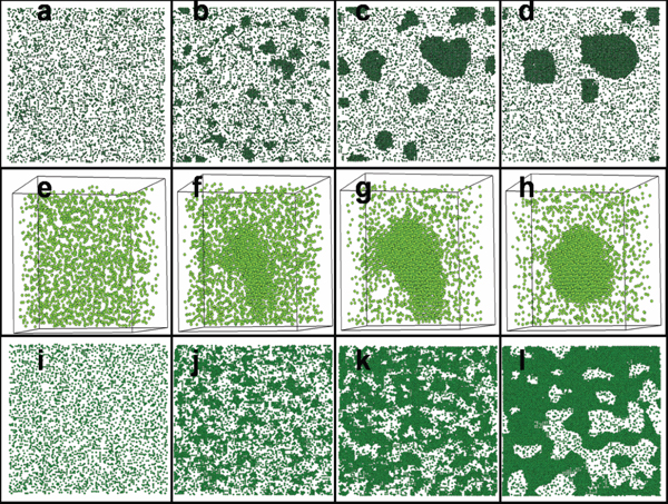
The described methodology is used
to study homogeneous precipitation of
α′ phase in saturated FeCr solution. The
study starts with the homogeneous case
at two compositions, x = 0.15 and x =
0.5, at T = 750 K, points identified with
stars in Figure 4; x = 0.15 is just above
the solubility limit, while x = 0.5 is well
within the spinodal. Figure 6 shows two-dimensional
slice sequences from MC
simulations that represent steps toward
equilibrium, starting from a solid solution
and evolving toward a segregated
state with α and α′ regions. All three
simulations correspond to perfect crystal
cubic samples with ~2 million atoms and
periodic boundary conditions.
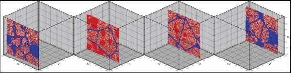
HETEROGENEOUS PRECIPITATION
In this study, heterogeneous precipitation
(i.e., precipitation in the presence
of defects) is explored in a polycrystalline
sample with average grain size of 5 nm. This enables the observation of a
multiplicity of configurations of grain
boundaries, triple and higher order
junctions, and eventually surfaces, in a
single run. Figure 7 shows four slices
taken at different locations in a cubic
sample represented by the boxes in the
figure. A surprising effect wherein the
excess chromium does not precipitate
at boundaries is observed. Instead all
α′ precipitates are in the grain interior,
avoiding contact with the grain boundary
network. Experiments reporting
grain boundary chromium depletion,26
presumably due to a kinetic effect
(vacancies migrating preferentially via
the chromium sites), do not allow one to
separate thermodynamics from kinetic
effects. Ab-initio results on free surfaces
predict no segregation.27 Since it is well
known that the good corrosion properties
of this alloy are due to formation of
chromium oxide at the surface, one can
conclude that in this alloy kinetic and
thermodynamic effects play significant
roles in the determination of the microstructure.
CONCLUSION
FeCr ferritic steels are candidate
materials for diverse applications in
advanced nuclear energy systems, from
cladding of fuel to structural components.
Recent ab-initio results have
shown that magnetism in these alloys
plays an important role in determining
its energetics at 0 K. The authors have
developed an approach to computationally
model processes in this system based
on a classical potential that captures the
essentials of its energetics and thermodynamics.
The tools developed allow
simulations of radiation damage collision
cascades, precipitation of saturated solutions,
and heterogeneous non-equilibrium
processes. We find that our potential
predicts rejection of chromium from
grain boundaries, an unexpected behavior
for the precipitation of the chromiumrich
solution. Thus FeCr is far from being
fully understood. Accurate simulations
can only be done if the intricate details
of its energetics and thermokinetics are
adequately captured. This work represents
a step into that direction.
ACKNOWLEDGEMENTS
This work was performed under the
auspices of the U.S. Department of Energy by the University of California,
Lawrence Livermore National Laboratory
under Contract No. W-7405-Eng-48,
with support from the Laboratory
Directed Research and Development
Program. At Los Alamos National
Laboratory this was supported by the
Advanced Fuel Cycle Initiative, NE-20.
REFERENCES
1. R.M. Martin, Electronic Structure. Basic Theory and
Practical Methods (Cambridge, U.K.: Cambridge
University Press, 2004).
2. G.J. Ackland, J. Phys. Cond. Matter, 14 (2002), p.
2975.
3. M.S. Daw, S.M. Foiles, and M.I. Baskes, Mater. Sci.
Rep., 9 (1993), p. 251.
4. A.E. Carlsson, Solid State Physics: Advances in
Research and Applications, vol. 43 (New York:
Academic, 1990).
5. P. Erhart et al., J. Phys. Cond. Matter, 18 (2006), p.
6585.
6. F.A. Garner, M.B. Toloczko, and B.H. Sencer, J. Nucl.
Mater., 276 (2000), p. 123.
7. A. Hishinuma et al., J. Nucl. Mater., 258-263 (1998),
p. 193.
8. S.J. Zinkle, Phys. Plasmas, 12 (2005), p. 058101.
9. A. Caro, D.A. Crowson, and M. Caro, Phys. Rev.
Lett., 95 (2005), p. 075702.
10. P. Olsson et al., J. Nucl.
Mater., 321 (2003), p. 84.
11. N. Saunders and A.P. Miodownik, Calphad. A
Comprehensive Guide, ed. W. Cahn Editor (Amsterdam:
Pergamon Materials Series, R., 1998).
12. I. Ansara and B. Sundman, Computer Handling
and Dissemination of Data (London: Elsevier Science
Pub Co., 1987).
13. A. Dinsdale, CALPHAD, 15 (1991), p. 317.
14. A. Caro et al., J. Nucl.
Mater, 336 (2005), p. 233.
15. A. Caro et al., J. Nucl.
Mater., 349 (2006), p. 317.
16. E.O. Arregui, M. Caro, and A. Caro, Phys. Rev. B, 66
(2002), p. 054201.
17. E.M. Lopasso et al., Phys. Rev. B, 68 (2003), p.
214205.
18. A. Caro et al., J. Nucl.
Mater., 323 (2004), p. 233.
19. A. Caro et al., Appl. Phys. Lett., 89 (2006), p.
121902.
20. M.I. Mendelev et al., Phil. Mag., 83 (2003), p.
3977.
21. J. Wallenius et al., Phys. Rev., 69 (2004), p.
094103.
22. T.P.C. Klaver, R. Drautz, and M.W. Finnis, Phys. Rev. B, 74 (2006), p. 094435.
23. A.A. Mirzoev, M.M. Yalalov, and D.A. Mirzaev, The
Physics of Metals and Metallography, 97 (2003), p.
336.
24. B. Sadigh et al., unpublished research (2006).
25. V. Barbe and M. Nastar, Nature Mater., 5 (2006), p.
482.
26. E. Wakay and et al., J. Physique, C7 (1995), p. 277.
27. W.T. Geng, Phys. Rev. B, 68 (2003), p. 233402.
A. Caro, M. Caro, and B. Sadigh are staff scientists
with the Chemistry, Materials, and Life Sciences
Directorate at Lawrence Livermore National
Laboratory in Livermore, California. P. Klaver is a
post doc at the School of Mathematics and Physics,
Queens University Belfast, Northern Ireland, United
Kingdom. E.M. Lopasso is a staff scientist at Centro
Atomico BarilocheInstituto Balseiro in Bariloche,
Argentina. S.G. Srinivasan is a staff scientist at Los
Alamos National Laboratory in New Mexico. Dr. A.
Caro can be reached at caro2@llnl.gov.
|
 Presenting a Web-Enhanced